Not everyone needs to be concerned with multi-channel attribution. If it makes up a very small part of your business, it might not be worth it. However, if you want to get a better understanding of the value of your traffic channels and the transactions/revenue they bring in, you might want to give it a go.
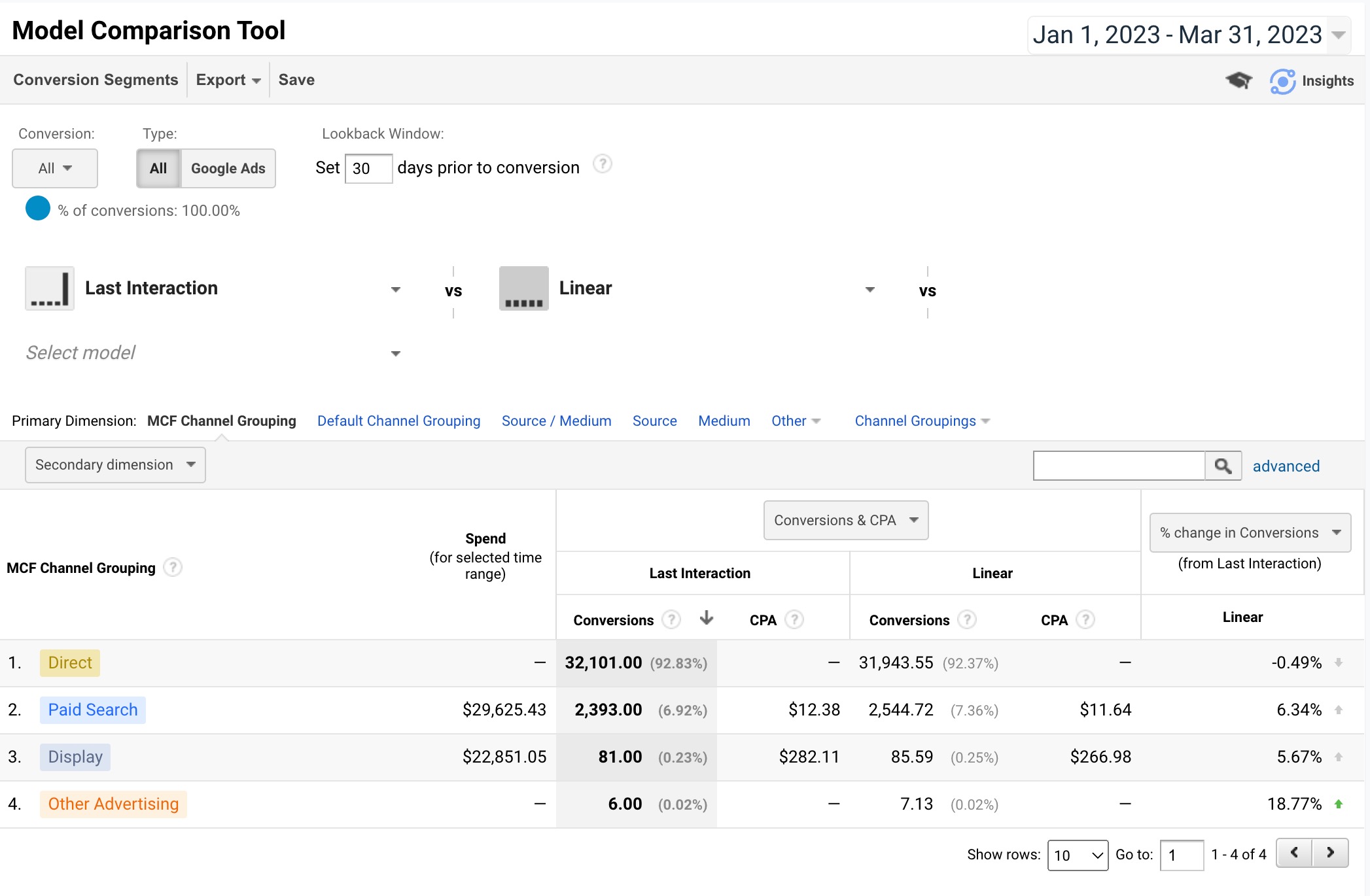
Using R Shiny to pull the raw data out of Google Analytics and create an app is one way to be able to explore your multi-channel attribution traffic channels. You might be asking yourself “if Google Analytics already provides this, why do I need anything else?”. That’s a good question and the answer is that Google Analytics will only calculate aggregated data over a single time period, not over a number of time periods. You miss out on trending over time. A second reason is that by building your own multi-channel app, you can decide how you want to calculate credit for each channel in the mix and you can see the credit calculations for yourself instead of having to rely on Google. In this app, I have given each channel equal credit. You can change this up by coding additional calculations – maybe even try a Markov Model.
I’m going to walk you through how to create a multi-channel attribution Shiny app using Google Analytics data in fifteen steps. It’s a bit advanced (believe it or not, it was the first Shiny app I created) but I will do my best to explain as much as I can and I will leave a Github link to the full, functioning (mostly – you do have to add your own Google Client ID & Secret) code as well as a link to a functioning app with sample data.
Step 1: Set Up Global Options
The first thing you want to do is get the data from Google Analytics. You will need to pull the data directly from Google Analytics. The best way is with the googleAnalyticsR package. But first, you will need a Google Client ID and Client secret.
To get a Google Client ID and Client secret, go to console.cloud.google.com. You will need to navigate to the OAuth consent screen. The User type is usually set as external. There are a couple other questions, such as setting user cap and token grant rate. Once you have finished with the OAuth consent screen, navigate to Credentials. You need to create an OAuth 2.0 Client ID. Simply click on “Create Credentials” at the top of the screen and select OAuth client ID. Name the ID and save. You should see your Google Client ID and Client secret in the upper right-hand column.
What I like to do from here is create a YAML file to store the IDs. It makes it easier to manage all the IDs for different data sources and they aren’t hard-coded into the app. A YAML file is simply a text file with a .yml extension. It’s easiest if you use the config package to access the YAML file. If you choose to use the config package, you’ll need to name it config.yml. Here’s what the file should look like inside (I’m using “GA”, but you can use “default”, it which case you won’t have to name the reference in the config::get() statement):
  GA:
    GA_CLIENT_ID: "YOUR CLIENT ID"
    GA_CLIENT_SECRET: "YOUR CLIENT SECRET"
Now that you’re setup with a Google Client ID and Client secret, as well as a YAML file, we’re ready to program a R Shiny app. We’re going to setup some global information for the app. To make it a little less confusing, I’m going to make this a single file app. It can be split into a global.R, ui.R and server.R, if you want. That makes sense with large apps.
We want to load the R packages we’re going to be using and load the Google Client ID and Client secret:
# Turns progress bar on or off.
progress = 1

# Load packages. Using pacman to make it easier,
# if a given package is missing.
if (!require("pacman")) install.packages("pacman")
pacman::p_load(shiny,
               googleAnalyticsR,
               googleAuthR,
               tidyverse,
               plotly,
               lubridate,
               plyr,
               shinythemes,
               rpivotTable,
               config)

# Using the config package to assign ga
# to GA in the config.yml file.
ga <- config::get('GA')

# Retrieving the GA Client ID and Client secret from
# the config.yml file.
options(googleAuthR.client_id = ga$GA_CLIENT_ID,
        googleAuthR.client_secret = ga$GA_CLIENT_SECRET)

# Authenticate and go through the OAuth2 flow first time -
# specify a filename to save to by passing it in.
gar_auth(token = "sc_ga.httr-oauth")

# At this point, you might want to
# retirieve the list of GA properties/views
# to get the View IDs you need.
account_list <- ga_account_list()
Step 2: Create Your UI
To create the user interface, you need three basic things:
- Page
- Row
- Column
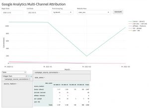
In this case, we are going to use one page. We are going to have the variables at the top of the page. Then we are going to have a time-series plot. Below that will be a pivot table. Both of these are interactive, to a degree.
# Assign the ui to a fluidPage(), which will
# display the output from server.
ui <- fluidPage(theme = shinytheme("lumen"),

          # Crate a title for when the app runs.
          titlePanel("Google Analytics Multi-Channel Attribution"),

          # I'm creating one row, with a column for each parameter.
          # These will be located at the top of the page.
          # A row can be divided up to 12 columns.
          fluidRow(
                  column(2,
                      dateInput("begin_date_select",
                                  "Begin Date:",
                                  min = as.Date('2018-01-01'),
                                  max = Sys.Date() - 1,
                                  value = Sys.Date() - 90)
                  ),

                  column(2,
                      dateInput("end_date_select",
                                  "End Date:",
                                  min = as.Date('2018-01-01'),
                                  max = Sys.Date() - 1,
                                  value = Sys.Date() - 1)
                 ),

                 column(2, # This one is whether the time-series
                           # should be by week or month.
                      selectInput("time_loop", "Time Grouping:",
                                  c("Pick one" = "0",
                                    "by Month" = "2",
                                    "by Week" = "1"))
                ),

                column(3, # This is a subset of the account_list
                          # variable created in the global section.
                          # You can subset it further, with dplyr::filter()
                          # if there are some views you don't want
                          # in the dropdown.
                      selectInput("ga_view_name", "Website View:",
                                   account_list$viewName)

                ),
                      br(), # A little space, then the button
                            # to run the code and get the data.
                      actionButton("goButton", "Calculate")
            ),

            fluidRow(

                  column(12,

                         # This will be the time-series output as a plotly plot.
                         # We will build this in the server section, with the
                         # name "distPlot".
                         plotlyOutput("distPlot", width = "100%", height = "100%")

                  )

            ),

            fluidRow(

                    column(12,

                           # This is the interactive pivot table, named
                           # "attribution_pivot" in the server section.
                           rpivotTableOutput("attribution_pivot", width = "100%")

                    )

            )

    )
Step 3: Create Your Server
This is section with the most code. We’re going to create this section, then get to work on a function to move from one time period to another, since we are using a time-series graph. This is the basic statement for the server:
server <- function(input, output){ # All our code is going in here }
All the code we will write will go between the curly brackets. The first function will be used later, but it’s vital to move from one time period to the next:
# For the selected time period, we have the beginning
# and end, but we need to loop through for each week/month
# so we can graph the trend in the Plotly time-series graph.
date_end_period <- function(date_select, time_select){

          # Check that the input variables are correct.
          stopifnot(time_select == 1 | time_select == 2)
          stopifnot(is.Date(date_select))

          # 1 for weekly / 2 for monthly.
          if (time_select == 1) {

                # Add the number of days until Saturday.
                output_date <- as.character(as.Date(date_select +
                                                (7 - wday(date_select))))

          } else {

              if (time_select == 2) {

                          # If it's the end of the year
                          # the next month will be 1 &
                          # and the year will be next year.
                          # Otherwise, just add 1 (year stays the same).
                          if(month(date_select) == 12){

                                    month_next <- 1
                                    year_next <- year(date_select) + 1

                          } else {

                                    month_next <- month(date_select) + 1
                                    year_next <- year(date_select)

                          }

                          # Put it all together, change to a date and then to character.
                          output_date <- as.character(as.Date(paste(year_next, "-",
                                                   month_next, "-01", sep = ""))-1)

                          return(output_date)

              }
        }
  }
Step 4: Configure Data Retrieval From GA Loop
This is the main work horse of the app. I’ve named it g_mca_data and it’s a reactive function to loop through the time periods, retrieving the multi-channel data for each and working through each dataset. A reactive function has global scope and only needs to be refreshed if the inputs change. We’ll be passing in the begin date and end date, which is the stop date for the function. We’ll also be passing in the time loop (whether the data should be retrieved by week or month) as well as the Google Analytics view name. Here is the code that will get the view id, end date for the first loop, and the setup for the loops:
g_mca_data <- reactive({

          # If the goButton hasn't been clicked,
          # don't run code.
          if(input$goButton == 0){return()}

          # Using the inputs from the UI.
          # isolate() prevents reevaluation.
          # Not really needed here due to above return()
          # but generally good to have when you don't
          # want your code reevaluated when an input variable changes.
          begin_date <- isolate(input$begin_date_select)
          stop_date <- isolate(input$end_date_select)
          time_loop <- isolate(input$time_loop)
          view_name <- isolate(input$ga_view_name)

          # Get the view id from the account list
          # from the view name that was selected in the UI.
          ga_id <- account_list %>%
                        dplyr::filter(viewName == view_name) %>%
                          dplyr::select(viewId)

          # Calculate the end date for the first period - call date_end_period().
          end_date <- date_end_period(begin_date, time_loop)

          # Calculate number of datasets to retrieve from GA.
          # We'll use this in the progress bar.
          diff <- difftime(stop_date, begin_date, units = 'weeks')

          # If it's months, divide by 4.
          # difftime() doesn't do months
          # and it doesn't have to be exact.
          if(time_loop == 2){

              diff <- diff/4

          }

          # This will be used by the progress bar.
          # It can be set from 0 - 1.
          loops <- 1/as.integer(diff)


          # Set dataframes we're going to use later to NULL.
          # They need to exist, but we don't need to assign
          # a value yet.
          ga_channel_attribution <- NULL
          ga_channel_attribution_final <- NULL

          # Inserting a progress bar to let users know how much longer.
          withProgress(message = 'Retrieving data', style = 'notification',
                       detail = 'fetching first dataset', value = 0, {

              Sys.sleep(0.25)

          # Open the loop and Loop through by week (or month).
          while (end_date <= stop_date) {
Step 5: Retrieve Google Analytics Multi-Channel Data
Once you have the function set up with the inital variables and are in the loop, to get multi-channel funnel data, you will need to use the google_analytics_3() function. This is because multi-channel funnel data is not available through the Google Analytics version 4 api.
# Get the GA source data - this will grab all transactions.
ga_conv_campaign <- google_analytics_3(ga_id,
                                       start = begin_date,
                                       end = end_date,
                                       metrics = c("totalConversions",
                                                   "totalConversionValue"),
                                       dimensions = c("campaignPath",
                                                      "sourceMediumPath"),
                                       filters = "mcf:conversionType==Transaction",
                                       samplingLevel = "WALK",
                                       type = "mcf")
As you can see, there are eight parameters. Some are fairly obvious (start, end) while others are not. The ga_id is the view id of the view from the property that you want to pull the data from. The metrics, in this case, are the number of conversions and the value of the conversions. Here, I am using the ecommerce transactions and value of the transactions. I’m also pulling in all the campaign combinations (campaignPath) that lead to conversions, each separated by a “>” (e.g. google / cpc > google / organic).
In this script, I want to know how each campaign performed – however, not every traffic source has a campaign attached to it. So I am also pulling in all the source/medium combinations (sourceMediumPath), each separated by a “>” as well. Next, I will take these two and merge them together.
Step 6: Create Function to Merge Campaigns and Sources
To merge the campaignPath and sourceMediumPath, I created a function to break down each string of campaigns and source/mediums, combining each individual source/medium/campaign. I am combining each source/medium with each corresponding campaign with a “–” (which we’ll use later to separate them out again, into their own columns). The reason to combine them together is that some campaigns are the same across source/mediums, so there needs to be a way to distiguish them and there can be a number of them in one row data.
# Input the campaign path and source path strings.
merge_source_campaign <- function (campaign, source) {

          # The # of campaigns and sources will be identical.
          # Set the # of campaigns from the campaign path string.
          campaign_source_count <- str_count(campaign, " > ") + 1

          # Split each of the strings by the campaign/source delimiter.
          campaign_split <- strsplit(campaign, " > ")
          source_split <- strsplit(source, " > ")

          # Convert the strings to matrixes, to reference each campaign/source.
          campaign_matrix <- matrix(unlist(campaign_split), ncol=campaign_source_count, byrow = TRUE)
          source_matrix <- matrix(unlist(source_split), ncol=campaign_source_count, byrow = TRUE)

          # Set the loop to the # of campaigns from the campaign path string.
          i <- campaign_source_count

          # Use a loop to work through the matrixes and replace
          # campaigns with the corresponding source/medium, "--", and campaign.
          while (i != 0) {

              campaign_matrix[1,i] <-
                  paste(source_matrix[1,i], campaign_matrix[1,i],sep="--")

              i <- i - 1

          }

          toString(campaign_matrix)

          # Replacing the ", " with the " > ".
          source_campaign_merge_str <- str_replace_all(toString(campaign_matrix), ", ", " > ")

          return(source_campaign_merge_str)

}
Step 7: Replace campaignPath With Source/Medium/Campaign
Loop through the the dataset, calling the merge_source_campaign() function above. This will merge each of the source/mediums in the sourceMediumPath with the corresponding campaign in the campaignPath.
# Work through the entire campaign attribution dataframe -
# replacing each campaignPath field with the returned
# source/medium/campaign value.
for(i in 1:nrow(ga_conv_campaign)){

          campaign <- ga_conv_campaign[i,1]
          source <- ga_conv_campaign[i,2]

          # Send the variables to the merge_source_campaign function,
          # return the updated campaign path string & replace the current
          # campaign path string with the updated one -
          # then move to the next row of data.
          ga_conv_campaign[i,1] <-
              merge_source_campaign(as.character(campaign), as.character(source))

}
Step 8: Remove Source/Medium/Campaigns That Should Not Be Credited For Conversions
We can drop the sourceMediumPath now, since it has been merged into the campaignPath. Also, we’ll remove direct visits that are not at the beginning of the string. This is because of the way I am thinking about multiple channels. If a visitor is coming back directly, the credit is going to the previous channel. If direct is first (it’s their first visit), then it is likely that they heard about the site somewhere offline – so we keep that one. You can manipulate this as you like. You have the option to credit sources/mediums/campaigns in the way that you think is right for your business.
# Create a new dataframe (there's more work ahead...).
ga_conv_source <-
        ga_conv_campaign %>%
                dplyr::mutate(campaign_path =
                              lapply(campaignPath,
                                     gsub,
                                     pattern = "> \\(direct\\) / \\(none\\): \\(unavailable\\)",
                                     replacement = ""),
                              total_conversions = as.integer(totalConversions),
                              total_conversion_value = as.numeric(totalConversionValue)) %>%
                tidyr::unnest(campaign_path) %>%
                dplyr::select(campaign_path,
                              total_conversions,
                              total_conversion_value)
Step 9: Calculate Number of Source/Medium/Campaigns For Each Set of Conversions
Calculate the number of source/medium/campaigns there are in each campaign_path and add that number as a separate column, as well as adding the fraction of conversions and conversion value for each source/medium/campaign. If you want to give more credit for the first/last source/medium/campaign, you can do that in the next step. If you want to to that, keep the total_conversions and total_conversion_value from the last step.
 # Add the number of campaigns.
ga_conv_source$campaign_source_count <- stringr::str_count(ga_conv_source$campaign_path, ">") + 1

# Calculate the fraction of conversions and conversion value for each
# campaign. Also, unnest the campaign_path lists - they are all lists.
ga_conv_source <-
        ga_conv_source %>%
            dplyr::mutate(campaign_source_conversions = total_conversions/campaign_source_count,
                          campaign_source_conversion_value = total_conversion_value/campaign_source_count) %>%
            dplyr::select(campaign_path,
                          campaign_source_count,
                          campaign_source_conversions,
                          campaign_source_conversion_value)
Step 10: Separate Each Source/Medium/Campaign Into Their Own Rows
Each source/medium/campaign will have a copy of their credit for the conversions and conversion value. If a campaign_path has only one source/medium/campaign, then it just needs to be copied over to the new dataframe. However, if there are multipe (as in multi-channel attribution), then they will have to be split out one at a time, then added to the new dataframe. This is where you can modify whether the first/last source/medium/campaign gets more credit for the conversions. It just takes a little bit of additional coding to mark the first/last and use the total_conversions and total_conversion_value to calculate the value for each source/medium/campaign, instead of using the campaign_source_conversions and campaign_source_conversion_value, which are meant for a linear calculation.
ga_attribution_channels <- NULL
i = 1

# Loop through ga_conv_source, separate all attribution
# channels with ' > ' as delimter and add each in the
# ga_attribution_channels table.
while (i <= nrow(ga_conv_source)){

        # If there is more than one source/medium/campaign, loop through them
        # and enter each into ga_attribution_channels
        # otherwise, move to the next row.
        if(ga_conv_source[i,'campaign_source_count'] > 1){

              # Set the temp table to null.
              ga_attribution_channels_temp <- NULL

              # Split out the source/medium paths into a character matrix.
              source_split <- str_split_fixed(ga_conv_source[i,"campaign_path"],
                                    pattern=fixed(' > '), n=Inf)

              e <- 1

              # Loop through the character matrix,
              # adding each source/medium and the associated values
              # to the temp dataframe.
              while(e <= length(source_split)){

                          # These are multiple source/mediums,
                          # so each source/medium takes 1/n of the orders & revenue.
                          source_split_fraction <-
                              data.frame(source_split[1,e],
                                 (ga_conv_source[i,"campaign_source_conversions"]),
                                 (ga_conv_source[i,"campaign_source_conversion_value"]))

                          # Rename source_split_fraction to match with ga_attribution_channels.
                          names(source_split_fraction)<-c("campaign_path",
                                                         "campaign_source_conversions",
                                                         "campaign_source_conversion_value")

                          ga_attribution_channels_temp <-
                                      rbind(ga_attribution_channels_temp, source_split_fraction)


                          # Move to the next source/medium/campaign.
                          e <- e + 1
              }

        } else{

              ga_attribution_channels_temp <-
                      ga_conv_source[i, c('campaign_path',
                                          'campaign_source_conversions',
                                          'campaign_source_conversion_value')]

        }

        ga_attribution_channels =
                   rbind(ga_attribution_channels, ga_attribution_channels_temp)

        i <- i + 1
}
Step 11: Group campaign_paths Together
Group all the campaign_paths together and add all the fractions of conversions and conversion values to get the totals for each source/medium/campaign across single channel as well as multi-channel attribution.
# Group by campaign_path - add what is now single source/medium/campaigns.
ga_attribution_channels <-
          ga_attribution_channels %>%
                dplyr::mutate(campaign_path = stringr::str_trim(campaign_path)) %>%
                dplyr::group_by(campaign_path) %>%
                dplyr::summarise(campaign_source_conversions =
                                        sum(campaign_source_conversions),
                                 campaign_source_conversion_value =
                                        sum(campaign_source_conversion_value))
At the end of each loop, you want to add the beginning and ending dates, add the data to the final dataframe that has all the time periods, and move to the next time period:
# Add the dates for this round.
ga_attribution_channels$begin_date <- begin_date
ga_attribution_channels$end_date <- end_date

# Add this dataframe to the final dataframe before next loop.
# This function will add the rows of the two dataframes together,
# provided that they have the same names and number of columns.
# Neat trick - since we declared ga_channel_attribution_final,
# even if it's NULL, it won't error, it'll just add the new dataframe.
ga_channel_attribution_final <-
    rbind(ga_attribution_channels, ga_channel_attribution_final)

# Adjust dates based on weekly or monthly loop.
# Here we call date_end_period(begin_date, time_loop)
# to figure out the next loop's end date.
begin_date <- as.Date(end_date) + 1
end_date <- date_end_period(begin_date, time_loop)

# If the start date is greater than the stop date (the end date from the UI),
# make the end date greater than the stop date by making it equal to the begin date.
end_date <- ifelse(begin_date > stop_date, begin_date, end_date)

# String to use in the progress bar to let
# the user know we're on to the next dataset.
date_select <- paste('Retrieving next data set: ', begin_date, ' to ', end_date, sep = '')

# Check to make sure we should display the progress bar,
# If so, assign the percentage completed (between 0-1) and
# display the date_select message above.
if(progress == 1){
    incProgress(loops, detail = date_select)
    Sys.sleep(0.25)}

} # End of loop.
That is the main section of code for the app and most of the ga_data_frame() function. There is still more to do, but this is where the heavy lifting ends.
Step 12: Separate Source, Medium, Campaign & Return Data
To extend this just a bit, we separate out the source, medium, and campaign into their own columns, so that those can be rolled up separately (this is where the “–” comes in handy). I also changed the campaign_source_conversions to integer to round off the fractions.
 ga_channel_attribution_finito <-
            ga_channel_attribution_final %>%
                        tidyr::separate("campaign_path",
                                      c("source", "medium"), sep = " / ") %>%
                        tidyr::separate("medium",
                                      c("medium", "campaign"), sep = "--") %>%
                        dplyr::mutate(campaign_source_conversions =
                                              round(as.integer(campaign_source_conversions), 0),
                                     campaign_source_conversion_value =
                                              round(campaign_source_conversion_value, 2),
                                     month = paste('M: ',
                                                   as.character(format(as.Date(begin_date),
                                                                       '%Y-%m')), sep = ''),
                                     medium_short = substr(medium, 1, 20),
                                     source_medium = paste(medium, source, sep = ' - '))

    return(ga_channel_attribution_finito)

} # End of function.
Step 13: Summarise Data
Now that we have the data for each time period, we need to summarise it for the pivot table. To do this, we are going to simply take the dataframe returned above and summarise by either week or month. I’ve called this function mca_data_out and here is the complete function:
mca_data_out <- function(time_input){

        # Retrieve the dataset created in g_mca_data().
        mca_output <- g_mca_data()

        # Time input is by week,
        # then group by begin_date,
        # which is the date of the
        # beginning of the week.
        if(time_input == "1"){

              mca_output <- mca_output %>%
                              dplyr::group_by(source_medium, begin_date) %>%
                              dplyr::summarize(campaign_source_conversions =
                                                 sum(campaign_source_conversions)) %>%
                              dplyr::ungroup() %>%
                              dplyr::rename(date_select = begin_date) %>%
                              dplyr::arrange(source_medium, date_select)

        }

        # If time input is by month,
        # group by month in the dataset.
        if(time_input == "2"){

                mca_output <- mca_output %>%
                                dplyr::group_by(source_medium, month) %>%
                                dplyr::summarize(campaign_source_conversions =
                                                   sum(campaign_source_conversions)) %>%
                                dplyr::ungroup() %>%
                                dplyr::rename(date_select = month) %>%
                                dplyr::arrange(source_medium, date_select)

        }

        return(mca_output)
}
Step 14: Create Time-Series Plot
We will use Plotly to create the time-series plot:
output$distPlot <- renderPlotly({

        # First, check if the goButton has been clicked.
        # If not, return.
        if(input$goButton == 0){return()}

        # We're retrieving the time period
        # selection, week or month.
        time_input <- isolate(input$time_loop)

        # Call mca_data_out to get the data.
        mca_data <- mca_data_out(time_input)

        # Output will be by week(1) or month(2).
        # This will determine the title of the x-axis.
        x_axis_title <- ifelse(time_input == "1", "Week", "Month")

        x_format <- list(

          title = x_axis_title

        )

        y_format <- list(

          title = 'Conversions'

        )

        # Draw the plot.
        mca_data %>%
               plot_ly( ., x = ~date_select,
                        y = ~campaign_source_conversions,
                        type = 'scatter',
                        mode = 'lines',
                        color = ~source_medium) %>%
                        layout(showlegend = TRUE,
                               autosize = T,
                               xaxis = x_format,
                               yaxis = y_format)

})
Step 15: Create Pivot Table
We will use rpivotTable to create the pivot table. This is a great function. Once the table is served, you can change the value inside to the table to be percentage of rows/columns or counts, etc. You can also remove source/mediums and filter by other variables that are passed in.
  output$attribution_pivot <- renderRpivotTable({

        # First, check if the goButton has been clicked.
        # If not, return.
        if(input$goButton == 0){return()}

        # We're retrieving the time period
        # selection, week or month.
        time_input <- isolate(input$time_loop)

        # Call mca_data_out to get the data.
        mca_data <- mca_data_out(time_input)

        # This will be the default value displayed
        # in the table.
        aggr_name <- 'Integer Sum'

        # Draw the interactive pivot table.
        rpivotTable(data = mca_data,
                    rows = 'source_medium',
                    cols = 'date_select',
                    vals = 'campaign_source_conversions',
                    aggregatorName = aggr_name)

})

} # Don't forget to close the server() function for the Shiny app.
So, in fifteen steps, you can create a multi-channel attribution Shiny app.
There are things that you might want to change (like the multi-channel attribution calculation, if you don’t like mine). This could be rewritten to get data day-by-day, then aggregate, without having to refetch the data. You may have also noticed that the output only uses the transactions and not the revenue. This can be changed around. Or when you are fetching the data, use a different conversion from GA.
You can check out the app with sample data from the Google Demo Account by clicking here to a shinyapps.io hosted version of the sample app.
I hope you enjoyed this post and it got you thinking about how to use Shiny apps to take GA to the next level. Here is the Github link to the full app code: https://github.com/daranjjohnson/multi_channel_attribution_ga_shiny